Java Architecture – How It Actually Works Under the Hood

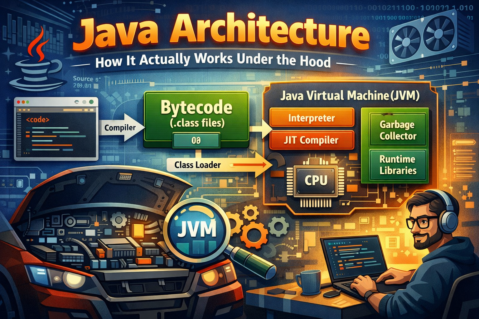
If you’ve been writing Java for a while, you’ve probably heard terms like JVM, JRE, JDK, bytecode, classloader thrown around. But how do these pieces actually fit together? What happens between the moment you hit Run and the moment your output appears?

This post walks through Java’s architecture from top to bottom — the way it actually works, not just the textbook definitions.

---

The Big Picture

Before getting into each component, here’s how everything connects:

flowchart TD
    A["📄 Source Code (.java)"] --> B["javac Compiler"]
    B --> C["📦 Bytecode (.class)"]
    C --> D["Class Loader"]
    D --> E["JVM Memory"]
    E --> F["Execution Engine"]
    F --> G["Interpreter"]
    F --> H["JIT Compiler"]
    G --> I["🖥️ Output"]
    H --> I

    subgraph JDK
        B
    end
    subgraph JRE
        D
        E
        F
    end

Java’s Write Once, Run Anywhere promise is built on one key idea: your code doesn’t compile to machine code directly — it compiles to bytecode, which the JVM then translates for whatever platform it’s running on.

---

JDK, JRE, JVM — What’s the Difference?

These three are often confused. Here’s a clean way to think about it:

graph TD
    JDK["JDK – Java Development Kit"]
    JRE["JRE – Java Runtime Environment"]
    JVM["JVM – Java Virtual Machine"]

    JDK --> JRE
    JRE --> JVM

Component	What it is	Who needs it
JVM	Executes bytecode	Everyone at runtime
JRE	JVM + standard libraries	Anyone running Java apps
JDK	JRE + compiler + dev tools	Developers

So when you install the JDK, you’re getting everything — the compiler (javac), the runtime (JRE), and the virtual machine (JVM). When you deploy to a server, usually only the JRE is needed.

---

Step 1 — Compilation

You write .java files. The javac compiler reads them and produces .class files containing bytecode. Bytecode isn’t machine code. It’s a platform-neutral instruction set that the JVM knows how to read. This is why the same .class file runs on Windows, Linux, or macOS without recompilation.

MyApp.java  →  javac  →  MyApp.class

---

Step 2 — Class Loading

Before the JVM can execute anything, it needs to load your .class files into memory. That’s the ClassLoader’s job.

flowchart LR
    A["Bootstrap ClassLoader<br>(loads rt.jar, core libs)"]
    B["Extension ClassLoader<br>(loads ext/ directory)"]
    C["Application ClassLoader<br>(loads your classpath)"]

    A --> B --> C

The loading process follows three steps:

1. Loading — reads the .class file and brings it into memory
2. Linking — verifies bytecode, allocates memory for static variables, resolves symbolic references
3. Initialization — runs static initializers and assigns initial values to static fields

One important thing to know: classloaders follow the parent delegation model. Before loading a class, a classloader asks its parent first. This prevents you from accidentally overriding core Java classes.

---

Step 3 — JVM Memory Areas

Once classes are loaded, the JVM organizes memory into distinct regions.

graph TD
    subgraph JVM_Memory ["JVM Memory"]
        A["Method Area<br>(class metadata, static vars, constants)"]
        B["Heap<br>(all objects live here)"]
        C["Stack<br>(per thread — frames, local vars)"]
        D["PC Register<br>(current instruction pointer)"]
        E["Native Method Stack<br>(for native/JNI calls)"]
    end

Method Area

Stores class-level data — field and method info, the bytecode itself, static variables, and the runtime constant pool. In modern JVMs (Java 8+), this is called Metaspace and lives in native memory (not the heap).

• Shared by all threads
• Created once when JVM starts
• Contains Runtime Constant Pool

Heap — Where Objects Live

The heap is shared across all threads. Every object you create with new ends up here.

flowchart LR
    subgraph Heap
        subgraph Y ["Young Generation"]
            Eden
            S0["Survivor 0"]
            S1["Survivor 1"]
        end
        O["Old Generation (Tenured)"]
    end

• Eden Space — new objects are allocated here first
• Survivor Spaces — objects that survive a minor GC get moved here
• Old Generation — long-lived objects eventually get promoted here
• Managed automatically by Garbage Collector
• Memory leaks mainly occur here

Stack — Where Method Calls Live

The Stack Area stores method execution information for each thread. Every method call creates a stack frame that holds local variables and references.

• Each thread has its own stack
• Stores local variables and method calls
• Memory is freed after method execution
• Faster than heap memory

Program Counter Register (PC) — Current Instruction Pointer

The Program Counter Register keeps track of the current instruction being executed by a thread. It helps JVM resume execution after thread switching.

• One PC register per thread
• Stores address of current JVM instruction
• Undefined for native methods
• Supports thread scheduling

Native Method Stack — For Native/JNI Calls

The Native Method Stack stores execution details of native methods written in languages like C or C++. It works alongside the Java Stack.

• Used for native (non-Java) methods
• Thread-specific memory area
• Depends on underlying OS
• Separate from Java Stack

---

Step 4 — Execution Engine

This is where bytecode actually gets run. The execution engine has two ways to do it:

flowchart TD
    B["Bytecode"] --> IE["Interpreter"]
    B --> JIT["JIT Compiler"]
    IE --> |"Slow but starts fast"| OUT["Native Machine Code"]
    JIT --> |"Fast after warmup"| OUT
    JIT --> PC["Profiling + Optimization"]

Interpreter

Reads and executes bytecode instructions one at a time. It starts up fast but is slower in the long run because it re-interprets the same instructions every time they’re hit.

JIT Compiler (Just-In-Time)

The JVM monitors which code runs frequently — these are called hot spots (that’s where HotSpot JVM gets its name). Hot code gets compiled to native machine code by the JIT compiler and cached. The next time that code runs, it executes at near-native speed.

This is why Java apps are slow to start but get faster as they warm up.

---

Garbage Collection — Memory You Don’t Have to Manage

Java handles memory deallocation automatically. The Garbage Collector (GC) periodically finds objects with no live references and reclaims their memory.

flowchart LR
    A["Object created in Eden"] --> B{"Survives Minor GC?"}
    B -- No --> C["Collected 🗑️"]
    B -- Yes --> D["Moved to Survivor Space"]
    D --> E{"Survives multiple GCs?"}
    E -- Yes --> F["Promoted to Old Gen"]
    E -- No --> C
    F --> G{"Old Gen full?"}
    G -- Yes --> H["Major GC / Full GC"]
    H --> C

Common GC Algorithms

GC	Good for	Trade-off
Serial GC	Single-threaded, small apps	Pauses everything
Parallel GC	Throughput-focused	Still causes pauses
G1 GC	Balanced, default since Java 9	Predictable pause times
ZGC / Shenandoah	Low-latency apps	Higher CPU usage

You can configure GC with JVM flags:

# Use G1 GC
java -XX:+UseG1GC -jar myapp.jar

# Use ZGC (Java 15+)
java -XX:+UseZGC -jar myapp.jar

---

Java’s Platform Independence — How It Actually Works

flowchart TD
    SRC["MyApp.java"] --> COMP["javac Compiler"]
    COMP --> BC["MyApp.class (Bytecode)"]
    BC --> W["JVM on Windows"]
    BC --> L["JVM on Linux"]
    BC --> M["JVM on macOS"]
    W --> WO["Windows Output"]
    L --> LO["Linux Output"]
    M --> MO["macOS Output"]

The bytecode is identical across platforms. Each platform just needs its own JVM implementation that knows how to translate that bytecode into the right native instructions.

---

Putting It All Together

Here’s the full end-to-end flow one more time, now with everything in context:

sequenceDiagram
    participant Dev as Developer
    participant Compiler as javac
    participant CL as ClassLoader
    participant MA as Method Area
    participant Heap as Heap
    participant EE as Execution Engine

    Dev->>Compiler: Writes .java file
    Compiler->>CL: Produces .class bytecode
    CL->>MA: Loads class metadata
    CL->>Heap: Allocates static objects
    Dev->>EE: Triggers execution (main())
    EE->>MA: Fetches bytecode
    EE->>Heap: Creates objects as needed
    EE->>Dev: Returns output

---

Quick Reference — Key Terms

Term	What it means
Bytecode	Platform-neutral compiled output of javac
JVM	Executes bytecode; platform-specific
JRE	JVM + standard libraries
JDK	JRE + dev tools (compiler, debugger, etc.)
ClassLoader	Loads .class files into JVM memory
Heap	Shared memory for all objects
Stack	Per-thread memory for method calls
Metaspace	Stores class metadata (Java 8+, native memory)
JIT Compiler	Compiles hot bytecode to native code at runtime
GC	Automatically reclaims memory from dead objects

---

Conclusion

Java’s architecture is what makes it both portable and performant. The JVM does a lot of heavy lifting behind the scenes — classloading, memory management, JIT optimization, garbage collection — so you can focus on writing clean application code.

Understanding this flow is genuinely useful beyond just interviews. When your app is slow to start, you know it’s JIT warmup. When you’re tuning memory, you know which heap region to look at. When you hit a ClassNotFoundException, you know exactly which layer broke.

---